Notes on Building a High-Precision Desktop Lathe

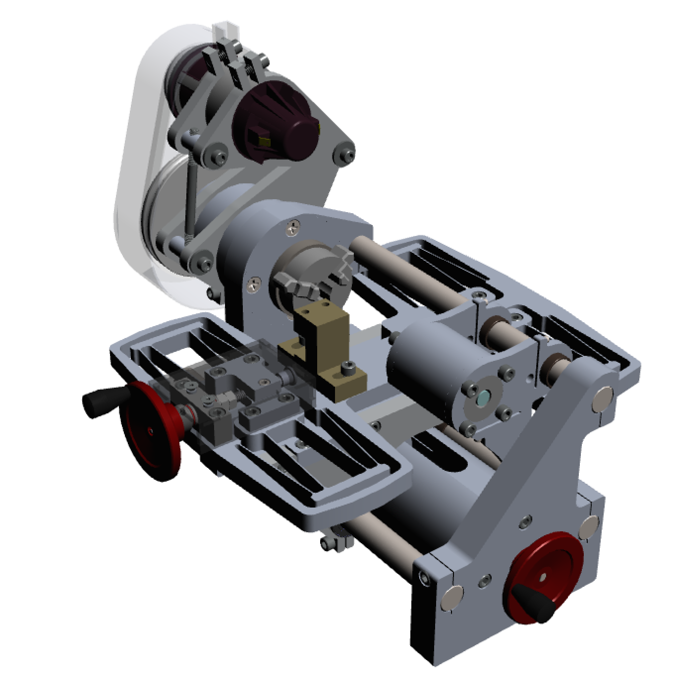
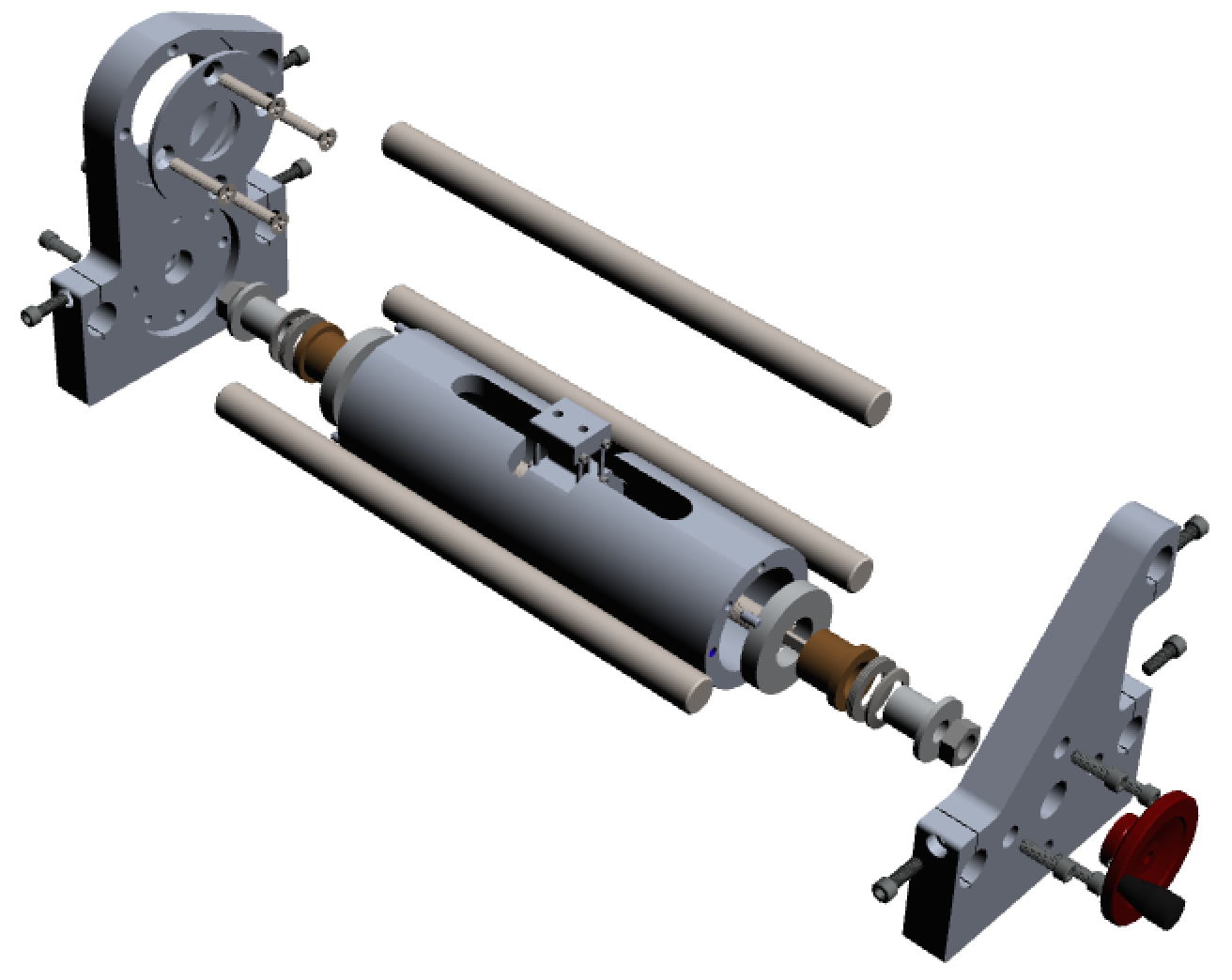
During my third year studying aeronautical engineering, I was fortunate enough to visit MIT on exchange. While there, I completed the 2.72 Elements of Mechanical Design course. The objective was to design and manufacture a high-precision desktop lathe using fundamental mech-E design principles.

As with most MIT courses, the lectures and course material are made publicly available on OpenCourseWare (OCW). Some students have also documented their experiences, see here, here, and here.

Rather than writing another blog detailing my experience taking the course, I'll focus on some interesting concepts I learnt along the way.

Using Transfer Matrices for Stiffness Calculations

The key metric that influences a lathe's quality is the workpiece-to-tool stiffness. There is a significant cutting force that traverses through the workpiece, via the spindle to the main lathe's structure and ends at the tool-piece.

But how do you calculate this?

One option could be to do an FEA, but this can be computationally expensive, and more importantly, time consuming, making iteration more challenging.

I was aiming to use a geometry-based ML optimization technique to evaluate all different structure configurations, so being able to quickly determine the overall system stiffness was needed. This is where Homogeneous Transfer Matrices (HTMs) come in!

As most Mech-E's do, I took a course on statics where we learnt how to calculate the stiffness of a beam under different load configurations.

Load Diagram	Equations
Axial Load	$d = \frac{FL}{EA}$
Cantilever Beam with Point Load	$d = \frac{FL^3}{3EI}, \;\; \theta = \frac{FL^2}{2EI}$
Cantilever Beam with Moment	$d = \frac{ML^2}{2EI}, \;\; \theta = \frac{ML}{EI}$

where $E$ is Young's modulus, $I$ is the second moment of area and $A$ is the cross-sectional area of the beam.

HTMs allow us to model the lathe as an inter-connection beams allowing us to calculate the relative deflection of a point relative to another based on a load vector.

For simplicity, I started with a 2D representation (this approach easily extends to the 3D case).

The deflection of $d$ relative to $c$ can be represented by

$$^d\mathbb{H}_c = \Bigg[ \; \begin{matrix} \cos(\theta) & -\sin(\theta) & -\delta _ 1 \\ \sin(\theta) & \cos(\theta) & H - \delta _ 2 \\ 0 & 0 & 1 \end{matrix} \; \Bigg]$$

Applying this to each beam element, the end-to-end HTM $^e\mathbb{H}_a$ can be calculated as

$$^e\mathbb{H}_a = \; ^e\mathbb{H}_d \cdot \; ^d\mathbb{H}_c \cdot \; ^c\mathbb{H}_b \cdot \; ^b\mathbb{H}_a,$$

and the 2D deflection vector

$$\mathbf{v} = \; ^e\mathbb{H}_a \cdot \Bigg[ \; \begin{matrix} 0 \\ 0 \\ F \end{matrix} \; \Bigg].$$

From this we can extract the

$$\mathbf{v}_y = \big[ \; \begin{matrix} 0 & 1 & 0 \end{matrix} \; \big] \cdot \mathbf{v}.$$

Now we have a function $\mathbf{v}_y = \mathcal{f}(F, L_1, L_2, H_1)$ which calculates the deflection as a function based on various design variables. By doing the same for $\mathbf{v}_x$ and $\mathbf{v}_z$ and any other deflection requirements, we can formulate an optimization function

$$\min_{L_1, L_2, H_1} \mathcal{f} \\ \text{s.t.} | L_1 | \leq ...$$

for a load profile $F$.

As usual, a key assumption is that deflections are small such that the geometry does not get significantly altered.

htms